UHIE modeling in Nicosia

UHIE modeling

Study objective: The objective of this study is to estimate the Urban Heat Island Effect (UHIE) of a location based on its characteristics and elevation, historical weather measurements from a reference station and temporal information. We approach UHIE modeling by decoupling the capacity of an area to exhibit a UHIE of a certain strength from the phenomenon excitation by ambient conditions.

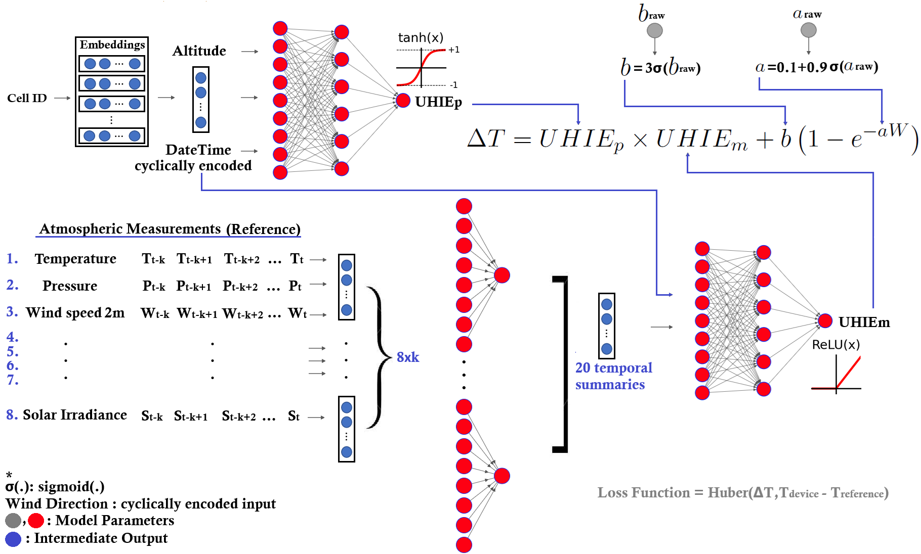
Core formulation: We use a quantity that represents the UHIE potential of each area (\(UHIE_p\)) and a quantity that represents the modulation of the UHIE sourcing from the ambient conditions (\(UHIE_m\)) such as temperature, humidity, wind speed at 2m and 10m above ground, wind direction, atmospheric pressure, and solar irradiance measured outside the urban fabric. Analyzing the phenomenon into these two discrete components makes its modeling easier, more accurate, and more interpretable. Concretely, we conceptualize the UHIE as follows: each area exhibits a potential \(UHIE_p\) to absorb and release heat which raises the temperature in its vicinity. The environmental conditions at a certain time modulate this potential resulting in a strengthening or weakening of its effect causing an analogous temperature increase. We model this interaction with \(UHIE_p\) in the range \((-1, +1)\) and \(UHIE_m\) in the range \((0, 1)\) because a landscape may have a positive or negative impact on the micro-climate while its modulation due to environmental conditions should be only positive or none. Formally: \[\Delta T = UHIE_p \times UHIE_m\] where \(\Delta T\) is the temperature variation from that measured outside but near the urban fabric.

Wind correction for mobile sensing: The accuracy of temperature measurements is significantly influenced by convective heat transfer, which is directly modulated by ambient wind conditions. Wind alters the thermal boundary layer surrounding the sensor, enhancing convective heat exchange between the sensor and the surrounding air. This effect can lead to either underestimation or overestimation of the ambient air temperature, depending on the sensor's design, response time, and radiation shielding. In our case, the sensors generally give lower readings due to convective cooling enhancement by high wind speeds. Since this measurement deviation is well within the range of temperature shifts expected due to the UHIE, the convective bias effect's magnitude is high enough to prevent meaningful results unless modeled. We add an extra term: \[\Delta T = UHIE_p \times UHIE_m + b \left(1 - e^{-aW}\right)\] where \(b \in [1,3]\) and \(a \in [0.1,1]\) are learnable parameters controlling the behavior of the convective effect, enforcing strictly negative effective values (cooling only). The parameters are computed as \(b = 3 \cdot \text{sigmoid}(b_{raw})\) and \(a = 0.1 + 0.9 \cdot \text{sigmoid}(a_{raw})\) to enforce valid value ranges.

Why 200 m × 200 m cells: The granularity of the study was chosen to be 200 m × 200 m cells to approximate the spatial scale of urban micro-climates and neighborhood blocks, at which built form and land cover characteristics (e.g., building density, vegetation cover, surface materials) are relatively homogeneous and directly relevant to human thermal exposure. A 200 m grid also aligns well with the spatial resolution of the input remote sensing data, allowing multiple satellite pixels to be aggregated within each cell to reduce noise while retaining sufficient spatial detail to capture urban thermal contrasts. Grid sizes of 200 m are commonly used in previous urban heat island studies.

Reference baseline and inputs: The record of environmental conditions at a given date and time, measured at a location just outside the urban area, was acquired from the Department of Meteorology, Section of Climatology and Applied Meteorology, Ministry of Agriculture, Rural Development and Environment of Cyprus. The weather station collecting these measurements every 10 minutes is located just outside the city center, in a sparsely built landscape with many trees and fields, which minimizes the development of the UHIE. Reference weather includes: temperature, humidity, wind speed at 2 m and 10 m above ground, wind direction, atmospheric pressure, and solar irradiance. Each in-city measurement is compared against this baseline to form the target \(\Delta T\). We also include the cell altitude and ID to capture orographic and spatial effects.

Time and date dependency: Another important aspect of our modeling is the assumption that UHIE is time- and weather-dependent. Our approach uses date and time as inputs, based on the premise that a location's UHIE potential varies significantly over the course of a day and across seasons. Similarly, the environmental conditions modulating this potential are also date- and time-dependent, as their impact is influenced by the specific time and date. This paradigm enables realistic modeling of the effect and captures the inherent complexity and dynamic nature of the phenomenon.

Temporal context (92 hours): The modulation term \(UHIE_m\) is driven by the recent history of weather because heat storage and release occur over many hours. We summarize the last 92 hours (nearly four days) of eight weather variables at 10-minute cadence. This window covers typical heatwave persistence and nightly cooling cycles. Extending the length of historical data beyond 48 hours appears reasonable, as prolonged conditions, such as heatwaves, play a significant role in UHIE, and the model should be able to track them. The history is later processed by learned temporal summaries to distinguish slow-accumulating heat from quickly dissipating conditions.

Filtering for data quality: Cells with fewer than 10 measurements are removed (119 cells) to avoid unstable estimates. This step was crucial to ensure sufficient statistical representation for each location in the dataset and thus consistency in the results. Mobile readings are averaged over 10-second windows to reduce sensor noise and GPS jitter. The combination of quality filters, reference baseline, and wind correction aims to deliver a stable estimate of \(UHIE_p\) and \(UHIE_m\) before we project to remote-sensing inputs.

Key takeaways: (1) Clear separation of intrinsic potential and weather modulation improves interpretability; (2) \(\Delta T = UHIE_p \times UHIE_m\) is the base, with an airflow cooling correction added; (3) 92-hour weather context captures accumulation and dissipation; (4) 200 m grid balances spatial detail with robustness; (5) Time and date encodings capture diurnal and seasonal variations.

AI for learning the UHIE potential

Model inputs: The AI model integrates the UHIE potential and its modulation with wind correction to compute the temperature difference between the 200 m cells and the reference temperature at a given time. The model's inputs include: the cell ID (an integer ranging from 0 to the maximum location index), the reference environmental parameters (temperature, humidity, wind speed at 2 m and 10 m above ground, wind direction, atmospheric pressure, and solar irradiance), as well as the wind speed and altitude measured by the vehicle-mounted device. Because the UHIE varies with both the time of day and the season, the model is also provided with the date and time of each measurement. During training, besides the UHIE potential, the model learns the vector descriptors (embeddings) of the various locations and the wind correction parameters \(a\) and \(b\).

Temporal processing with 20 summary channels: The model computes the UHIE modulation by considering the historical environmental conditions provided by the weather station outside the urban fabric, specifically the measurements taken over the last \(k=92\) hours. These measured quantities influence the extent to which the UHIE potential at a given location translates into a temperature difference. Certain environmental conditions during the last \(k\) hours, such as high temperature and lack of wind, facilitate the accumulation of heat in materials, thereby strengthening the effect. To enable the model to compute an appropriate temporal mixing of this historical information, we use 20 linear layers, each capable of assigning its own weight to each measurement time step, thus forming 20 temporal summaries for the UHIE modulation estimation. For example, one temporal summary might assign great importance to the last 24 or 12 hours, while another might apply a cyclic preference, focusing on the last 6 hours, the first 12 hours, and an interval in between. Since reference measurements are available every 10 minutes, the full historical input is \(8 \times 92 \times 6 = 4416\) values.

Cyclic encoding for periodic variables: Several inputs to the model exhibit an intrinsic periodic structure. Wind direction angle, calendar date, and time of day all repeat after a fixed cycle. In such cases, representing these variables in a linear numerical form introduces an artificial discontinuity at the boundaries of the cycle—for instance, 359° and 0° represent nearly identical wind directions, and 23:59 is temporally adjacent to 00:00, yet linear encoding treats these values as maximally distant. To preserve the true topological and geometric relationships within these variables, we apply a cyclic (circular) encoding scheme. Each periodic variable \(x\), defined over a period \(Q\), is embedded in a two-dimensional representation using \((\sin(2\pi x/Q), \cos(2\pi x/Q))\). This transformation maps the variable onto the unit circle, eliminating discontinuities at cycle boundaries and ensuring that semantically adjacent values are also close in the encoded feature space.

Model outputs and network architecture: The network predicts \(UHIE_p\) through a \(\tanh\) head (range [−1, 1]) and \(UHIE_m\) through a ReLU head (non-negative). The two fully connected Neural Networks (NNs) utilized by the model to compute the UHIE potential and modulation have a hidden layer of size 128, use the Rectified Linear Unit (ReLU) as activation in their hidden layer, and have a single output. The NN computing the UHIE potential utilizes the hyperbolic tangent function (\(\tanh\)) at its output producing UHIE potential values in the range \([-1,1]\) while the NN computing the UHIE modulation uses a ReLU function at its output to ensure that the estimated value is positive. A 64-dimensional embedding per cell is learned jointly, capturing the thermal behavior of the location.

Training objective and loss function: During training, the model computes UHIE potential and modulation based on its parameters, the date and time of the measurement, the wind speed recorded by the car-mounted equipment, and the location's attributes. These results are combined in the equation to calculate the difference between the temperature measured by the car-mounted device at a given location and the reference temperature. The model's loss function is the Huber loss between the predicted temperature difference \(\delta T\) and the ground truth: \[L_\delta(y, \hat{y}) = \begin{cases} \frac{1}{2}(y - \hat{y})^2 & \text{if } |y - \hat{y}| \le \delta \\ \delta \cdot (|y - \hat{y}| - \frac{1}{2}\delta) & \text{otherwise} \end{cases}\] Huber loss is employed because it is less sensitive to outliers than other regression functions like mean squared error (MSE), reducing the risk of destabilizing training due to erroneous values. Notably, the temperature measurements within the urban area taken by the car-mounted equipment are not used by the model to compute the components of the equation—instead, they are used to construct the ground truth values used in the loss function.

Data preprocessing and training details: We use simple preprocessing on all measurements acquired by the car-mounted equipment and the weather station. Specifically, we apply min-max normalization to the measurements to enforce a value range between 0 and 1: \(x' = \frac{x - \min(x)}{\max(x) - \min(x)}\). This improves training dynamics and prevents numerical instabilities and feature dominance, ensuring that no single measurement disproportionately influences the learning process due to its scale. We trained the model with the AdamW optimizer, a learning rate of 0.001, and a weight decay of 0.0002. The size of the locations' embeddings was chosen to be 64, which offered enough expressivity to the model to fit the data but not too much space to overfit it. We split the dataset into training and validation sets, using 90% of the datapoints for optimizing model parameters and the remaining 10% to validate results.

Key implementation notes: (1) Temporal-summary diversity (~40.5) confirms the model uses multiple historical regimes; (2) Training Huber loss reached 0.13 with validation loss of 0.145; (3) 863 location embeddings are learned; (4) Constrained parameters keep airflow correction physical.

Datasets

Vehicle-mounted measurement system: A vehicle-mounted device was developed to collect spatially resolved temperature and wind speed measurements during real-world driving. The system records geographic position and auxiliary contextual variables simultaneously. All sensing, processing, and storage functions are integrated into a compact, self-contained unit suitable for extended mobile operation. Conducting environmental measurements from a moving vehicle poses several challenges, including aerodynamic disturbances and radiative heating effects. The systematic biases introduced by these effects are negligible in stationary measurements but become significant under mobile conditions. Therefore, the system emphasizes physical separation between sensors and heat-generating components, controlled exposure to ambient airflow, and consideration of air speed caused by car movement.

Hardware architecture: The central controller is a Raspberry Pi 4 module (RPi4) that manages sensor polling, time-stamping, and local data logging, ensuring consistent temporal alignment across all measurement channels. Three TMP117 high-precision digital temperature sensors (±0.1°C accuracy within -20°C to +50°C range) provide measurement redundancy and 16-bit resolution (0.0078°C). A SEN0170 cup anemometer (0–30 m/s range, IP65 rated) positioned downstream of the temperature sensors measures airflow directly impacting them. A TEL0137 USB GNSS receiver provides 1 Hz geo-location updates with 2.5 m circular error probable (CEP). An RV-8803 real-time clock (±3 ppm accuracy) maintains precise timestamps during power interruptions. Measurements are recorded locally on a micro SD card with geographic coordinates and timestamps.

Data acquisition campaign: Two measuring devices were developed to support two independent missions each day throughout August and September: one during the morning to early evening hours (08:00–15:00) and one during the evening to nighttime hours (18:00–23:30). The car routes were not explicitly scheduled for data acquisition purposes—municipality employees performed their regular duties while simultaneously collecting data. They mounted devices on the car roof before their shift started, removed them at the end of their shift, and charged equipment batteries when necessary. The data acquisition phase resulted in approximately 700,000 data points, based on the 1-second acquisition interval configured for the devices. A larger dataset could have been obtained were it not for the summer break of the car crew and operational constraints requiring frequent stops to perform assigned tasks.

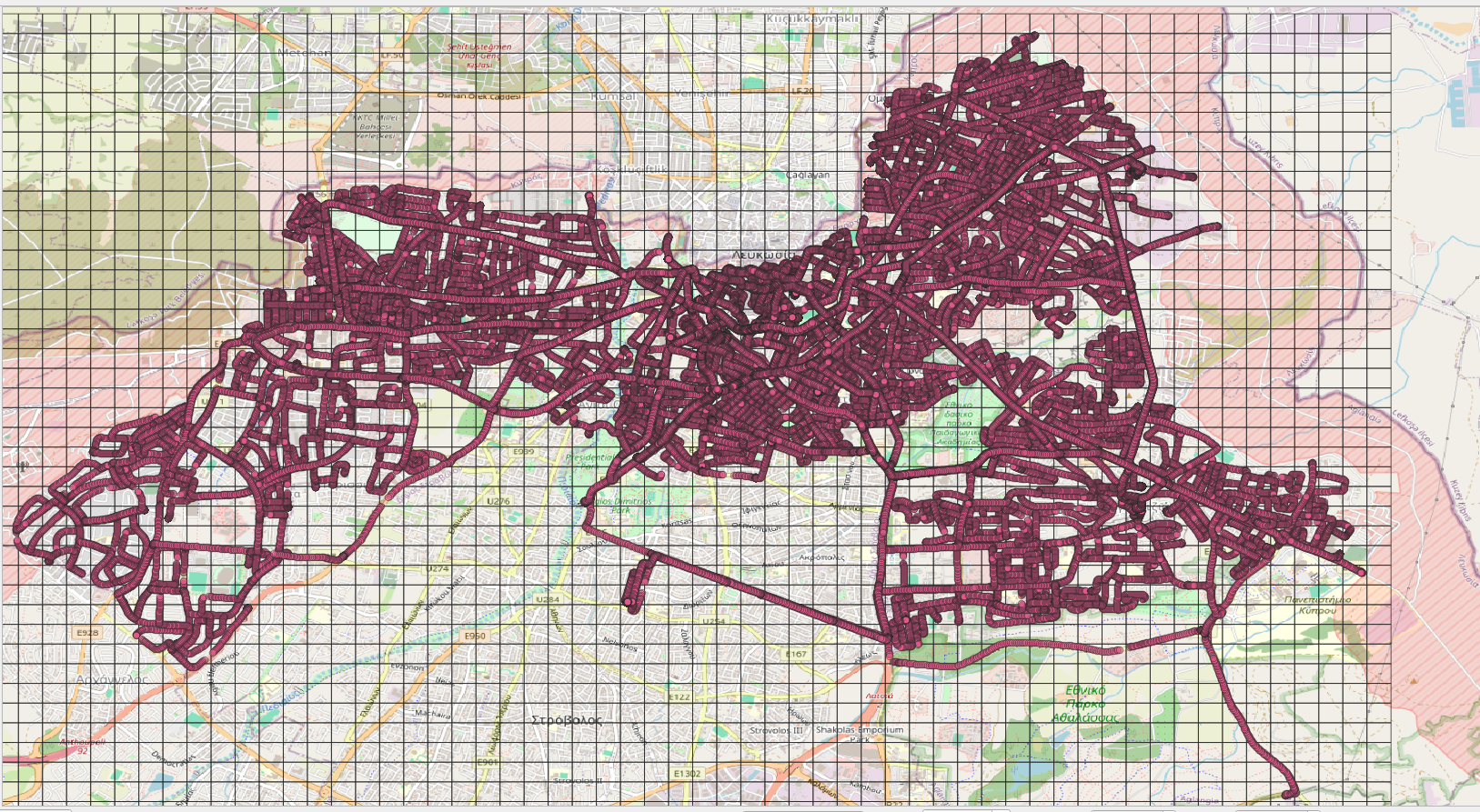
Spatial coverage of measurements: The map below shows all temperature measurement locations recorded over the course of the data acquisition phase. Each point corresponds to a single measurement captured by vehicle-mounted equipment. The collected dataset comprises measurements spanning an area of approximately 8 km², obtained along different vehicle routes and at various times of day. Due to limited resources, data collection was not fully systematic—meaning temperature at a given location was not always measured repeatedly across different days and times. The model's ability to generalize helps mitigate this dataset limitation.

Reference station: The Athalassa weather station, operated by the Department of Meteorology of Cyprus, is located just outside the city center in a sparsely built landscape with many trees and fields, which minimizes the development of the UHIE. It provides the baseline at 10-minute cadence for temperature, humidity, wind speed at 2 m and 10 m above ground, wind direction, atmospheric pressure, and solar irradiance. \(\Delta T\) targets are computed as (mobile temperature − reference temperature) at matched timestamps. Using an out-of-city baseline reduces contamination from local UHIE and keeps the target consistent.

Weather history for modulation: Eight weather quantities over the last 92 hours feed the modulation term \(UHIE_m\). This window spans nearly four days, capturing heatwave buildup, overnight cooling, and wind-driven dissipation. With measurements every 10 minutes, the full input is \(8 \times 92 \times 6 = 4416\) values. Temporal summaries (learned) combine these histories differently so the model can respond to both slow and fast atmospheric regimes.

Third-party validation data: To validate our results, we used data from Weather Underground and its WunderMap platform—an interactive, real-time weather visualization platform that integrates data from a global network of personal and professional weather stations. We focused on temperature and wind speed measurements from six stations located in areas (200 m cells) visited by our data acquisition vehicles during data collection: IAGLAN3 (Aglantzia area), IENGOM5 and IENGOMI3 (Engomi area), INICOS12 (Nicosia center), and ISTROV12 and ISTROV17 (Strovolos area). We developed a script to access data tables for each day of the vehicle data acquisition period (August to October 2025) and automatically extract temperature and wind speed measurements at five-minute intervals.

Remote sensing layers: While not downloaded here, the RS predictor consumes high-resolution satellite RGB imagery, spectral bands (including Near-infrared NIR for material identification), AI-inferred building height maps, and tree detection mapping to regress to the learned thermal embeddings. The 200 m grid aligns the RS pixel stack with the learned UHIE representation, allowing multiple satellite pixels to be aggregated within each cell.

Results

Training performance: Model training resulted in a Huber loss of 0.13, with a slightly higher validation loss of 0.145. During training, we monitored the sum of the mean absolute differences between all pairs of the 20 summary channels, anticipating a high value that would indicate the model is extracting distinct and diverse features from the measurement history. Consistent with this expectation, the diversity of the temporal summaries was high, reaching 40.5 in the final training epoch. After training was completed, we collected the UHIE potential for all 863 locations across the times of day and months covered by the study, namely from August 1 to October 10, between 07:00 and 23:00. Specifically, the trained model was used to compute the UHIE potential for every location at hourly intervals.

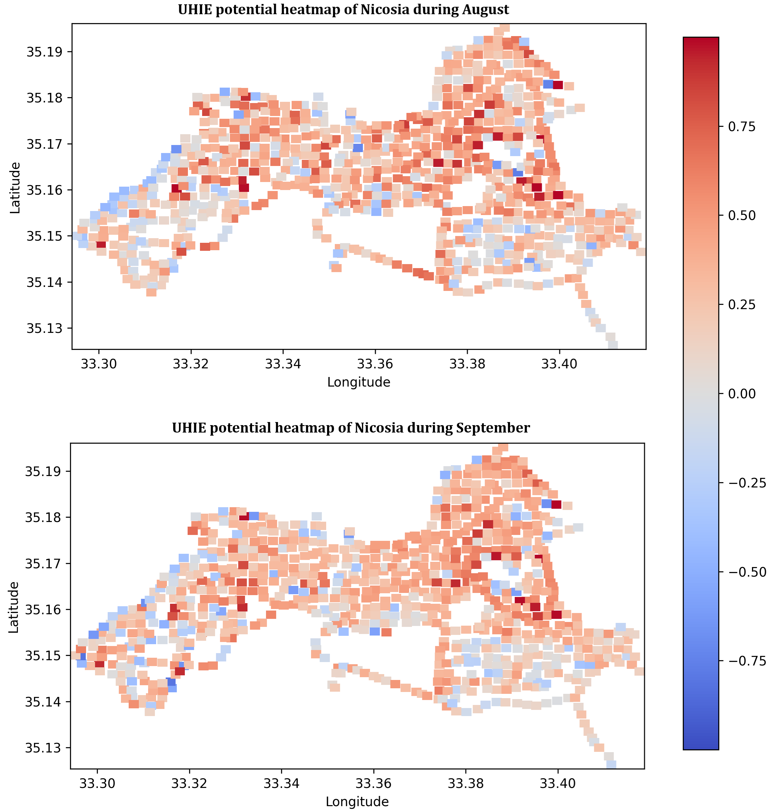
Spatial UHIE potential maps: We constructed two UHIE heatmaps for the city of Nicosia, one for August and another for September, by averaging the computed potential values across all times of day for each location for the specific months. While averaging across times of day suppresses the dynamic nature of the UHIE potential modeling—namely the temporal variation of the potential—the plots nevertheless capture a valuable aspect of the phenomenon's spatial distribution. The maps illustrate the intrinsic potential of an area to influence the temperature in its vicinity, either by increasing or decreasing it relative to the reference temperature measured outside the urban area. A location exhibiting a low potential (indicated by the blue color spectrum) does not necessarily experience lower temperatures than those measured outside urban regions during all times.

Interpreting the potential values: The potential is modulated by the environmental conditions of the preceding \(k\) hours, which may amplify it, resulting in substantial positive or negative temperature deviations, or attenuate it altogether. Furthermore, because the depicted potentials represent values averaged over times of day for each location within a given month, the displayed maps do not reflect the UHIE potential at all times of day—the actual potential varies over the course of the day and across days within the month. To compute a location's UHIE potential at a specific time of day and date, we use the model by providing as inputs the cell ID, the location altitude, and the date and time encoded using a cyclic representation. Since the model learned each location's intrinsic characteristics during training (64-dimensional embedding), it requires only the location's index, altitude, and temporal information to compute its UHIE potential.

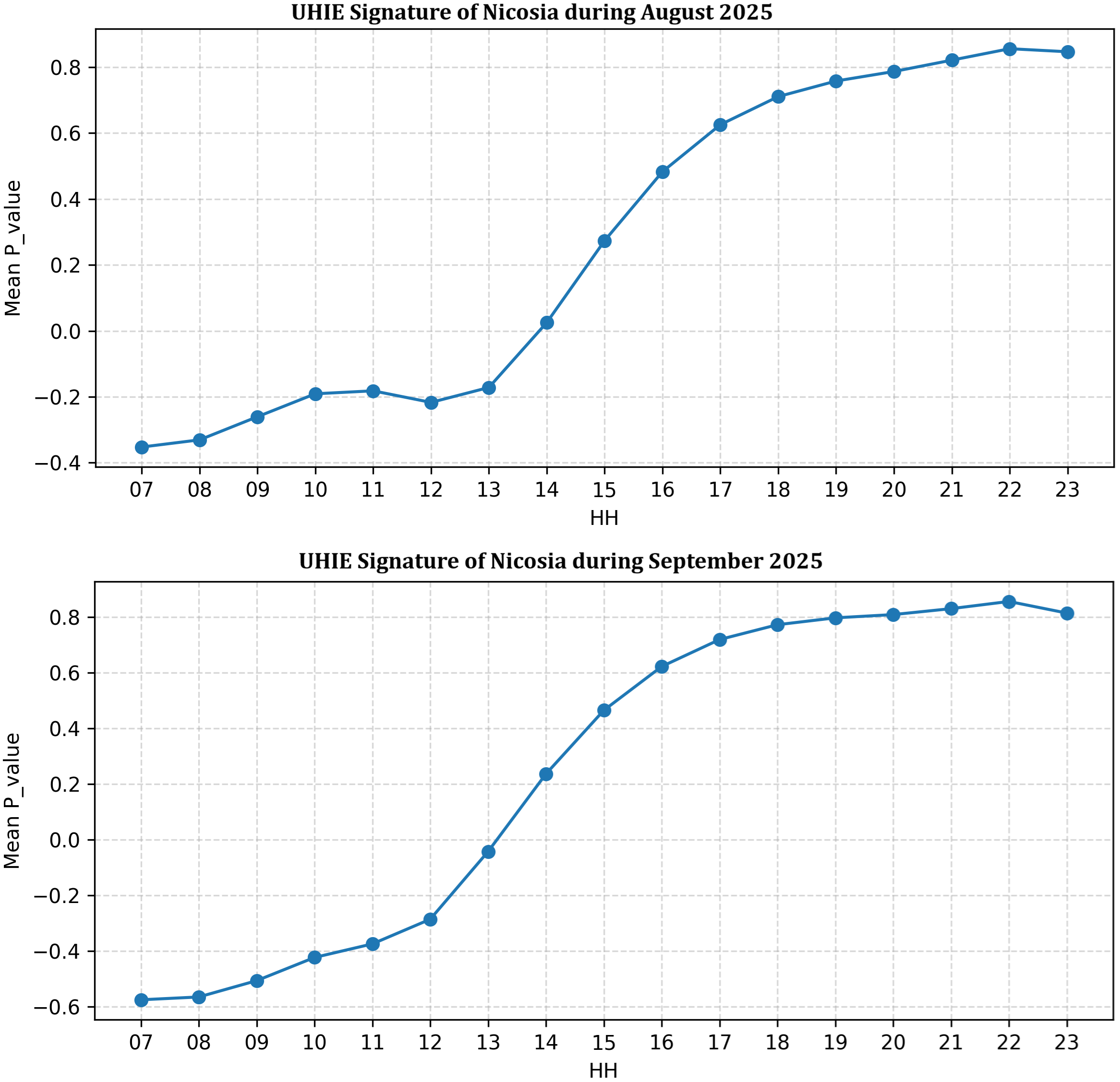
City signatures (diurnal patterns): Another notable insight derived from the UHIE potentials is the UHIE signature of the city. This visualization depicts the characteristic temporal pattern of UHIE potential across the urban area. It is generated by averaging the potentials over all days of a given month at different hours and represents the typical variation of UHIE throughout the hours of the day. This signature effectively captures the distinctive daily profile of the city, revealing when the city is most prone to express stored heat and how that shifts across months.

Validation with Weather Underground stations: We validated the model using measurements from six independent Weather Underground stations. For each station, we computed the Mean Absolute Error (MAE) and mean bias. Results show that the model consistently overestimates stations' temperature (mean bias positive for all stations), which is expected because the model is trained to predict temperatures for locations on asphalt surfaces and thus inherently accounts for the increased UHIE associated with such environments. The consistent upward difference suggests that the model outputs would align with station measurements if the additional UHIE of the asphalted surface were removed. Validation MAE ranged from 0.25°C (ISTROV17) to 1.09°C (IENGOMI3), demonstrating robust performance despite temporal and spatial sparsity of the mobile acquisition data.

Conclusion

Reserved for future updates.

Vehicle-mounted Equipment

Design requirements and objectives: The primary objective was to develop a compact, vehicle-mounted sensing platform capable of capturing spatially referenced environmental data for UHIE analysis. The design requirements included: (i) frequent (every 1 second) multi-point temperature acquisition with high precision (±0.1°C), (ii) wind speed measurement for mitigating the convective heat transfer effect, (iii) accurate geolocation tagging of all measurements (~1 m resolution), (iv) precise timestamping independent of network connectivity for robustness, (v) low power consumption suitable for extended mobile operation, (vi) a durable enclosure for outdoor deployment resilient to direct sunshine, prolonged vibrations and mechanical stresses, and (vii) safe vehicle mounting that prevents damage to the vehicle and ensures the safety of users and bystanders.

System architecture: The system employs a sensor array built around a Raspberry Pi 4 (RPi4) Model B single-board computer. Four distinct sensing modalities are integrated via RPi4's I²C and USB interfaces, enabling simultaneous acquisition of temperature, wind speed, temporal and positional data. The RPi4 was selected as the processing unit due to its robust Linux-based operating system and extensive peripheral connectivity options. Its quad-core ARM processor provides sufficient computational power for real-time data processing and logging, while the standardized I²C and USB interfaces simplify sensor integration. The overall hardware architecture has a modular design in which sensors, auxiliary systems, storage, power system and processing unit are placed in different compartments but are tightly synchronized.

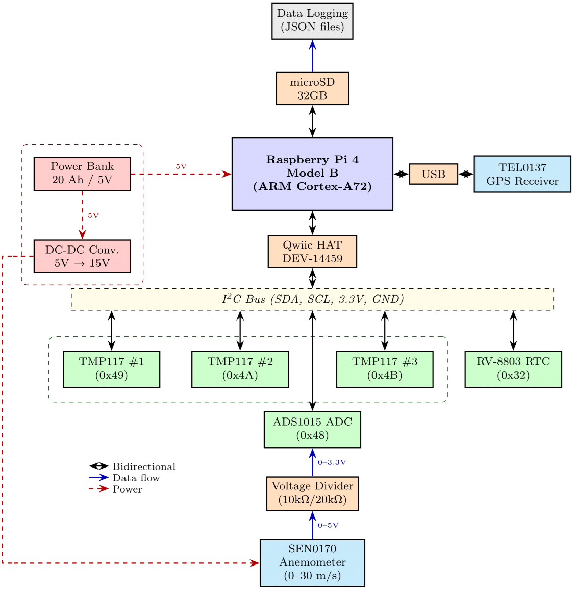
Temperature measurement subsystem: Temperature sensing is achieved using three SparkFun TMP117 high-precision digital sensors. The TMP117 was selected based on its superior accuracy specification of ±0.1°C within the -20°C to +50°C range, which is a critical requirement for detecting subtle thermal gradients characteristic of urban microclimate variations. Each sensor provides 16-bit resolution (0.0078°C), enabling the detection of fine-scale temperature differences between measurement locations. The deployment of three temperature sensors provides measurement redundancy for quality assurance. During data analysis, the individual readings are averaged to produce a single representative temperature value for each observation, thereby reducing random measurement noise. The sensors' ultra-low power consumption (3.5 µA typical) makes them suitable for maintaining a low overall system power budget.

Wind speed measurement subsystem: To measure wind speed, we use a SEN0170 by DFRobot cup anemometer sensor, which provides a linear analog voltage output (0–5V) corresponding to wind speeds ranging from 0 to 30 m/s (0 to 108 km/h). The SEN0170 is rated IP65 (ingress protection), rendering it suitable for outdoor mobile deployment. Wind speed data are used to characterize the convective heat exchange conditions during measurements, which significantly influence temperature readings. The anemometer is positioned immediately downstream of the temperature sensors within the airflow path between the air inlets and outlets. This design choice enables accurate measurement of the airflow directly impacting the temperature sensors. The anemometer requires an external DC power supply (9–24V) separate from the main system power, addressed through a DC-DC boost converter.

Positioning subsystem: Geo-location is provided by a TEL0137 USB Global Navigation Satellite System (GNSS) receiver, which acquires GPS signals at a 1 Hz update rate and achieves a circular error probable (CEP) of 2.5 m. Its USB interface facilitates integration with the RPi4, while the receiver is managed via the standard gpsd daemon, a background service on Unix-like systems that provides abstracted NMEA sentence parsing and a well-documented Python API. This positioning subsystem enables precise geo-referencing of all environmental measurements, supporting subsequent spatial analysis and mapping of thermal variations.

Timekeeping subsystem: The RPi4 relies on software-based timekeeping, which can drift noticeably when network access is limited or unavailable. This issue is particularly problematic for mobile devices that traverse long distances and frequently encounter connectivity interruptions. To address these limitations, we use an RV-8803 real-time clock (RTC) module. Unlike the RPi4's internal clock, the RV-8803 maintains high precision (±3 ppm, approximately ±0.26 s per day) without any reliance on external synchronization. A compact CR1225 backup battery keeps the RTC operational during power interruptions, such as battery swaps or recharging, ensuring uninterrupted timestamping.

Interface design and signal conditioning: The SparkFun Qwiic HAT module provides a standardized interface between the RPi4's GPIO-based I²C bus and the Qwiic-compatible peripheral sensors. This ecosystem employs polarized 4-pin JST connectors carrying 3.3V power, ground, and the I²C data (SDA) and clock (SCL) signals, enabling daisy-chain connectivity and tool-free assembly. A significant design challenge arose from I²C address conflicts—both the ADS1015 ADC and TMP117 temperature sensors default to address 0x48. This conflict was resolved through hardware modification of the TMP117 sensor boards, reconfiguring their addresses to 0x49, 0x4A, and 0x4B respectively. The anemometer's 0–5V output exceeds the 3.3V maximum input voltage of the ADS1015, so a resistive voltage divider (R1=10kΩ, R2=20kΩ) conditions the signal to the ADC's input range.

Power system design: The system's total power budget was evaluated to ensure compatibility with a portable power bank. The RPi4 accounts for the majority of power consumption (3–6.4W depending on processor load), whereas all I²C sensors together draw less than 10mW due to their low-power design. The GPS module consumes approximately 250mW, and the anemometer requires up to 400mW at 12V. The total system power ranges from 4–7W. Using a high-capacity (20 Ah) power bank simplifies device handling and provides greater operational flexibility. The power bank is housed in an easily accessible compartment, allowing operators to remove, charge, and replace it with minimal effort.

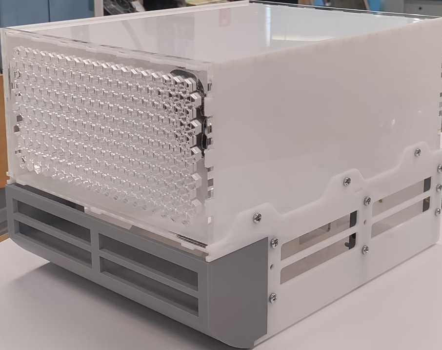
Mechanical integration and enclosure: The electronics assembly is housed within a 3D-printed enclosure, providing protection against dust and water jets—conditions expected during vehicle-mounted outdoor operation. The enclosure base was fabricated using a toughened polylactic acid (PLA) filament while the other parts were fabricated using polymethyl methacrylate (PMMA). The enclosure consists of two separate compartments: a lower section containing the main circuitry (RPi4, interfacing logic, GPS, RTC, and power electronics) and an upper section housing the temperature sensors and the anemometer. The upper compartment allows airflow through a front air inlet and a honeycomb structure that reduces turbulence and directs the flow toward the temperature sensors, then the anemometer, and finally through the outlet. Positioning the sensors and anemometer at the top of the assembly minimizes aerodynamic interference from the vehicle body. Additionally, the temperature sensors are shielded from direct solar radiation and positioned to sample ambient airflow representative of the surrounding environment.

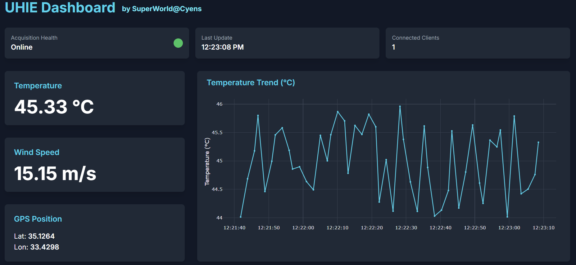
Software architecture: The data acquisition software is implemented in Python 3, leveraging manufacturer-provided libraries for I²C device communication (Qwiic Python packages) and the gpsd-py3 library for GPS data access. The software architecture employs a multi-threaded design with separate acquisition loops for each sensor subsystem, synchronized through a common timestamp derived from the RTC. Acquired data is logged to JSON files with timestamps and GPS coordinates, facilitating subsequent geospatial analysis, and stored on an onboard SD card. Device operators can monitor the data acquisition process in real time on their mobile devices (smartphones or tablets) via a locally hosted web page on the RPi4 module. This reporting tool allows for early detection of potential issues and actively engages operators in the process, enabling them to provide valuable insights based on their observations.

Bill of materials summary: The complete system costs approximately €494 (excluding 3D printing materials and consumables). Key components include: DFRobot SEN0170 anemometer (€49.40), three SparkFun TMP117 sensors (€48), SparkFun ADS1015 ADC (€18), SparkFun RV-8803 RTC (€19.50), SparkFun Qwiic HAT (€7), DFRobot TEL0137 GPS receiver (€12.50), TI DC-DC converter (€17.20), four car suction cup mounts (€220), and a 20000mAh power bank (€62).